Lab 2: Radiometric and Atmospheric Correction

Goal and Background:

The goal of this lab is to go through the process of correcting remotely sensed images for atmospheric interference. Multiple methods of correction will be used, Empirical Line Calibration, Dark Object Subtraction, and image normalization models.



Methods:

The first method of atmospheric corrections used was the Empirical Line Calibration method.  To begin, the image was brought into ERDAS Imagine and the spectral analysis workstation was opened.  From the workstation, the spectral signatures for various different areas of the image.  When taking the spectral signatures, the built in spectral libraries were referenced and selected as spectral references.  This means that each signature taken from the image, will be corrected using the previously corrected spectral signature from the same object, water, concrete etc. The Spectral Analysis Workstation then provides the regression equation for each of the bands for their spectral signatures.  The numbers from these equations are then used in the formula used to correct the image.  ELC is done using the following equation.  ERDAS Imagine has a built in tool that does this equation to your image for you, once the spectral signatures are taken. The user selects View-Preprocesses-Atmospheric Adjustment and it runs the image through the following equation and produces an output image that is atmospherically corrected. 

The next method used was the Dark Object Subtraction method.  This method takes a number of parameters into consideration when correcting the image.  It accounts for sensor gain, offset, solar irradiance, solar zenith angle, atmospheric scattering, absorption and path radiance.  This data is obtained from metadata that comes with the image as well as a few constants.  The DOS method consists of two steps, conversion to at-satellite spectral radiance and then from at-satellite spectral radiance to true surface reflectance.

The first step of this process begins with running each band of the image through the following equation. 

Qcalmin, Qcalmax, LMIN, and LMAX are all obtained from the images metadata.  The equation was performed on the image by using the model builder in ERDAS.  It was performed separately for each band.

Once the model was complete, all the bands were stacked into one image.  It was now ready to convert from at-satellite radiance to true surface reflectance.  This was done the same way as the other conversion but with a different equation and different variables.

Many of these values are gained from the metadata and other sources online.  They are ran on the image using a model that looks very similar to the first step.  The following image the equation.  A few values changed for each band.

The output of the model was images for each band so once again, the bands needed to be stacked into one image.  This is now an image that is atmospherically corrected using the DOS method.

The next part of the lab was to do relative atmospheric correction using multidate image normalization.  This is done by taking two images from different periods of time and collecting spectral samples from the same location in both images.  This was all done using the spectral profile tool in ERDAS.  The signatures were taken over a variety of different land features to ensure variability.  The following image is the resulting spectral profiles for the image from 2000 and 2009.

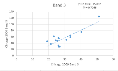
The profiles are slightly different for each image.  The next step is to take the mean pixel values for each band for each of the samples, for each image and use them to create a chart that includes the regression equation.  This was done using the table in ERDAS and bringing the values into Excel.

These values were then combined for the image from 2000 and the image from 2009, 2009 was the  X-axis and 2000 was the Y-axis.  Using Excel the slope equation was calculated for each band.

This slope equation was then used to as the inputs in the following equation.

The equation was ran on each band using a model in ERDAS.

The bands were then combined into one normalized image.




Results:
The following image is the image corrected using DOS and the original image.  The pane on the right is the original and the left is the corrected.  The corrected image is more sharp to the eye but you can really tell a difference when the spectral signatures are examined.  The spectral signatures are much closer to their known signature than before. 

The next image is comparing the ELC and the DOS corrected images.  The image on the left is the ELC and the right is the DOS.  The DOS is more clear and the spectral signatures are more accurate.  This means the DOS method was more successful in conducting atmospheric corrections.  This is possibly due to using more in situ data about the image and more values are inputted that change for each band.                                                                                                                                                                                                                                                                                                                             

The resulting spectral signatures for the normalized image when compared to the image from 2000 were similar but different in a few bands.


Sources:

Cyril Wilson
Landsat

Lab 1: Surface Temperature Extraction

Goal and Background:

This lab is designed to introduced the workflow of extracting land surface temperature information from thermal bands of satellite images and account for variations in land surface temperature over space. This lab will take satellite imagery and run it through two models in order to get surface temperature in radiance not in true temperature.  A later lab will introduce the workflow to produce true temperature of surface features.


Methods:

When thermal bands come straight from the source, they do not give surface temperature right away.  Some manipulation needs to be done to the imagery.  This is done by doing two different calculations to the images.  The first calculation is to get the spectral radiance readings at the sensors aperture. The equation is visible below.  It consists of multiplying the rescaled gain with the image band then adding on the rescaled offset.  The gain and offset are obtained by looking at the sensors metadata.  In order to get the Grescale or gain, a simple equation is used.  All this information can be gained from the image metadata.

Figure 1

This at aperture conversion equation can be seen in the image below (figure 2) for band 62 of a landsat ETM+ image of the Eau Claire Wisconsin area. The equation is from figure 1 with the proper values for grescale and brescale plugged in as well as the image bands. Once this is ran, another conversion needs to be done in order to get the blackbody surface temperature.

Figure 2

The following equation (figure 3) is the equation to convert the at satellite radiance to blackbody surface temperature.  Tb is at satellite temperature in kelvin, K1 and K2 are pre launch satellite constants that can be obtained online or from the metadata and the L value is the spectral radiance which is gained from the first conversion that was done. 

Figure 3

The following image (figure 4) is the above equation with the right numbers plugged in.

Figure 4

Results:

The resulting image is after running both conversions on the Landsat ETM+ Eau Claire image from the year 200.  This image was brought into ArcMap and symbolized.  From this image, surface temperature can be found by using the identify tool in ArcMap.  Note that these surface temperatures are in Kelvin.  A simple conversion needs to be done in order to get the temperature in fahrenheit or  celcius.  Now these temperatures are not the true kinetic surface temperatures.  To get true surface temperature, the material each object the earth is made of needs to be taken into consideration.  This method also assumes the unity of emissivity and uses pre-launch constants.

Figure 5

The final figure (figure 6) is a image of the surface temperature in Eau Claire and Chippewa county taken from the Landsat 8 Satellite.  This image was put through the same process as the other image but using the correct constants.

Figure 6

This method is a quick and easy way to extract surface temperature from thermal remote sensed data.  there is more steps needed to get true surface temperatures that will be highlighted in future labs.

Sources:

Cyril Wilson
Landsat